Day 2: Statistics and Probability Basics

In this blogpost, we will be amplifying our area of focus on Statistics and Probability, which plays a crucial role in the field of Data Science and Machine Learning. We will also have a look at some of the algorithms and will also look into the practical application of it.

Concept of Descriptive Statistics

Descriptive statistics summarize and organize data so it’s easier to understand. Think of it as a way to describe the data’s main features. You might be familiar with the concepts such as “Mean“, “Median“ and “Mode“. Well, that is that comes under it.

Mean is basically average of data.

Median is nothing but the middle value after the dataset is sorted.

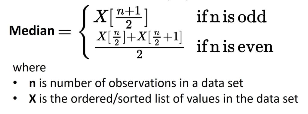
We use the following way to calculate the Median:

• Arrange data values from lowest to highest value (Sort them out)

• The median is the data value in the middle of the set

• If there are 2 data values in the middle the median is the mean of those 2 values.

Considering data array as [10,20,30,40], the median is 25. Because as there are 2 values in between 20 and 30, the Median will be 25 in our case. If the dataset is like [10,20,30,40,50], then the median will be 30.

Mode is the value which appears more frequently in the dataset than the other ones.

For instance, if our dataset is [10,20,20,30,40], then the Mode for the same is 20, as this value makes more apperance than the rest.

Measures of Dispersion

Measures of dispersion comes in action to showcase how much spread, or how much variable the dataset is. We will be looking at 3 of them in this blogpost: Range, Variance and Standard Deviation.

Range is the difference between the maximum and minimum values.
For Example: Condider a dataset [10,20,30,40,50,60,70].

Now as per formula : Range of above dataset = 70-10 = 60

Variance measures how far the data points are from the mean (average).

Next is Standard Deviation. It is basically the square root of variance, representing data spread.
Example: A dataset with a high standard deviation means the data points are spread out

Probability

Guessing that many peeps know about the “Probability“, we will just have a slight look as part of a formality.

In simple words Probability quantifies the likelihood of an event occurring.

Now there are 3 key terms associated with the concept of Probability. They are Experiment, Outcome and an Event. A Dice example as always is excellent in order to understand the concepts.

Experiment is a process leading to an outcome (e.g., rolling a die). Outcome is a possible result (e.g, rolling the number 6) and and Event can be best described as the collection of outcomes (chances of rolling an even number).

Bayes’ Theorem

Bayes’ Theorem calculates the probability of an event based on prior knowledge of related events.

Practical Implementations

Time for practical implementations in Python. I repeat, Python language will be instrumental for us in upcomming blogs, so it is the matter of utmost importance that one must get a good hands-on understanding of Python Language.

Here is an example of the concepts of Descriptive Statistics.

import numpy as np

data = [10, 20, 30, 40]

# Mean
mean = np.mean(data)
print(f"Mean: {mean}")     # Mean: 25.0

# Median
median = np.median(data)
print(f"Median: {median}")  # Median: 25.0

# Standard Deviation
std_dev = np.std(data)
print(f"Standard Deviation: {std_dev}")  # Standard Deviation: 11.18

Now let us look an another example we saw earlier, the probablity of Dice rolling an even number.

# Probability of rolling an even number
favorable_outcomes = 3  # {2, 4, 6}
total_outcomes = 6
probability = favorable_outcomes / total_outcomes
print(f"Probability of rolling an even number: {probability}")     # 0.5

Take a note, we are considering only 1 Dice, not 2.

Last but not the least, here is an example of Bayes’ Theorem implemented in Python.

# Known probabilities
P_D = 0.01  # Probability of having the disease
P_Pos_D = 0.95  # Probability of testing positive if diseased
P_Pos_not_D = 0.05  # Probability of testing positive if not diseased
P_not_D = 1 - P_D  # Probability of not having the disease

# Total probability of testing positive
P_Pos = (P_Pos_D * P_D) + (P_Pos_not_D * P_not_D)

# Bayes' Theorem
P_D_given_Pos = (P_Pos_D * P_D) / P_Pos
print(f"Probability of having the disease given a positive test: {P_D_given_Pos:.4f}")  # 0.1613

You might well just test them manually by the formaulae mentioned above, or you may use Python code snippets to do the job.

Conclusive Notes

• Descriptive Statistics help summarize data using measures like mean, median, and standard deviation.

• Probability quantifies the likelihood of events and follows key rules (addition, multiplication, complement).

• Bayes’ Theorem allows for updating probabilities based on new evidence, a critical concept in machine learning.

Well that concludes the lesson for today. I know most of the peeps/readers are itching to dive in the advanced concepts parts such as Generative AI , RAGs and LLMs, but trust me, once we got an overview on basics thoroughly, we will find the concepts much more easy.

Practice the concepts above with different examples and gain a clearer understanding.

Until then, Happy Learning!!