
Meta Description: Learn statistical analysis in R with hands-on examples. Understand hypothesis testing (t-test, ANOVA, chi-square), p-values, correlation, and simple and multiple linear regression using the built in mtcars dataset.
Introduction
Imagine a food delivery app that proudly claims: “Your order arrives in 30 minutes on average.”
You have ordered from it many times, and it feels like it always takes longer. But is your feeling real, or did you just get unlucky a few times? Your friends say the same thing, but a few complaints do not prove anything. To settle this fairly, you would need a method:
- Start by assuming the company is telling the truth (average is 30 minutes)
- Collect real delivery times from many orders
- Ask: “If the company’s claim were true, how surprising would my data be?”
- If the data would be extremely surprising, you reject the claim. If not, you cannot say it is false
That is the heart of hypothesis testing. The company’s claim is the null hypothesis, your orders are the sample, and “how surprising is my data” is the p-value.
Now suppose you also notice that the farther the restaurant is, the longer the delivery takes. You would love to say something precise like: “Every extra kilometer adds about 3 minutes.” Putting an exact number on a relationship like that is what regression does.
Today, we use R to do both: test claims with data, and measure relationships between variables. These are the tools that turn raw numbers into defensible conclusions, which is exactly what we need for tomorrow’s case study.
Theory and Brief History
Hypothesis testing helps you decide whether a pattern in your sample is real or just chance, and regression helps you measure how one variable changes when another changes.
- 1900: Karl Pearson introduced the chi-square test for comparing categorical data.
- 1908: William Sealy Gosset, a brewer at Guinness who needed to test small batches of beer, published the t-test under the pen name “Student”, because his employer did not allow staff to publish under their names. That is why it is called Student’s t-test.
- 1920s: Ronald Fisher popularized the p-value and developed ANOVA (Analysis of Variance).
- 1886: Francis Galton coined the term “regression” after noticing that tall parents tend to have children closer to average height, which he called “regression toward the mean.” The mathematical method behind it, least squares, goes back to Legendre and Gauss in the early 1800s.
Hypothesis Testing: Key Vocabulary
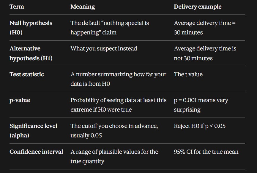
A p-value is not the probability that the null hypothesis is true. It is the probability of seeing data this extreme assuming the null hypothesis is true. This is one of the most commonly misunderstood ideas in all of statistics, and interviewers love to test it.
Two Kinds of Mistakes
- Type I error (false positive): rejecting H0 when it is actually true. Its probability is alpha.
- Type II error (false negative): failing to reject H0 when it is actually false. Its probability is beta, and power = 1 - beta.
Which test to use?
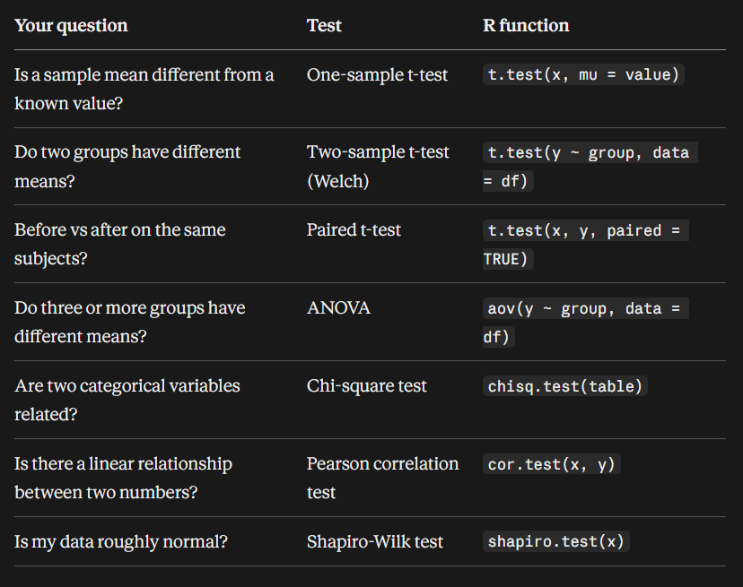
If data is clearly not normal, non parametric alternatives exist, such as wilcox.test() and kruskal.test(). In Python, the same tools live in scipy.stats and statsmodels.
Regression in a nutshell
Simple linear regression fits a straight line:
y = intercept + slope * x
- Intercept: the predicted y when x is 0
- Slope: how much y changes for each one unit increase in x
- Multiple regression uses several predictors:
y = b0 + b1*x1 + b2*x2 + ..., and each coefficient is interpreted holding the other variables constant
Reading the model summary:
- Estimate: the fitted coefficient
- Std. Error, t value, Pr(>|t|): tell you whether that coefficient is significantly different from zero
- R-squared: the share of the variation in y explained by the model (0 to 1)
- Adjusted R-squared: R-squared corrected for the number of predictors, so adding useless variables does not look like an improvement
- Residual standard error: the typical size of prediction errors, in the units of y
Assumptions of linear regression (remember the word LINE):
- Linearity: the relationship between x and y is linear
- Independence: observations do not depend on each other
- Normality: residuals are roughly normally distributed
- Equal variance (homoscedasticity): residuals have constant spread
Correlation does not imply causation. Cars with larger engines may have lower mileage, but regression alone cannot prove the engine size is the cause.
Practical
As in Days 27 and 28, use Posit Cloud, a Colab notebook with an R runtime, or a local R setup. We use the built in mtcars dataset (32 cars, from a 1974 magazine road test), so no file download is needed. Key columns: mpg (miles per gallon), wt (weight in 1000 lbs), hp (horsepower), cyl (cylinders), and am (transmission: 0 = automatic, 1 = manual).
Expected outputs are shown under each cell. Tiny differences in formatting between R versions are normal.
Cell 1: Explore the data
head(mtcars, 3)
               mpg cyl disp  hp drat    wt  qsec vs am gear carb
Mazda RX4     21.0   6  160 110 3.90 2.620 16.46  0  1    4    4
Mazda RX4 Wag 21.0   6  160 110 3.90 2.875 17.02  0  1    4    4
Datsun 710    22.8   4  108  93 3.85 2.320 18.61  1  1    4    1
Cell 2: Descriptive statistics for mileage
mean(mtcars$mpg)
sd(mtcars$mpg)
summary(mtcars$mpg)
[1] 20.09062
[1] 6.026948
   Min. 1st Qu.  Median    Mean 3rd Qu.    Max.
  10.40   15.43   19.20   20.09   22.80   33.90
Always describe your data before testing it. The average car here gets about 20 mpg.
Cell 3: Compare average mileage by transmission
tapply(mtcars$mpg, mtcars$am, mean)
       0        1
17.14737 24.39231
Automatic cars (0) average about 17.1 mpg, while manual cars (1) average about 24.4 mpg. Is this gap real, or just luck from a small sample? Hypothesis tests will tell us.\
Cell 4: Check normality with the Shapiro-Wilk test
shapiro.test(mtcars$mpg)
	Shapiro-Wilk normality test

data:  mtcars$mpg
W = 0.94756, p-value = 0.1229
H0 here is “the data is normal.” Since p = 0.1229 is above 0.05, we do not reject H0, so treating mileage as roughly normal is reasonable.
Cell 5: One-sample t-test
t.test(mtcars$mpg, mu = 20)
	One Sample t-test

data:  mtcars$mpg
t = 0.08506, df = 31, p-value = 0.9328
alternative hypothesis: true mean is not equal to 20
95 percent confidence interval:
 17.91768 22.26357
sample estimates:
mean of x
 20.09062
H0: the true mean mileage is 20. The p-value of 0.93 is huge, so we have no evidence against it. Notice the 95% confidence interval (17.9 to 22.3) contains 20, which agrees with this conclusion.
Cell 6: Two-sample t-test (automatic vs manual)
t.test(mpg ~ am, data = mtcars)
	Welch Two Sample t-test

data:  mpg by am
t = -3.7671, df = 18.332, p-value = 0.001374
alternative hypothesis: true difference in means between group 0 and group 1 is not equal to 0
95 percent confidence interval:
 -11.280194  -3.209684
sample estimates:
mean in group 0 mean in group 1
       17.14737        24.39231
H0: both transmission types have the same average mileage. With p = 0.0014 (below 0.05), we reject H0. The confidence interval for the difference does not include 0, so manual cars in this dataset are significantly more fuel efficient. R uses Welch’s version by default, which does not assume equal variances in both groups.
Cell 7: Chi-square test for two categorical variables
tbl <- table(mtcars$cyl, mtcars$am)
tbl
chisq.test(tbl)
    0  1
  4  3  8
  6  4  3
  8 12  2

	Pearson's Chi-squared test

data:  tbl
X-squared = 8.7407, df = 2, p-value = 0.01265

Warning message:
In chisq.test(tbl) : Chi-squared approximation may be incorrect
Rows are cylinders (4, 6, 8) and columns are transmission (0, 1). H0: cylinders and transmission type are independent. With p = 0.013, we reject H0, since 8 cylinder cars are mostly automatic. The warning appears because some expected counts are below 5. In practice, fisher.test(tbl) is a safer choice here.
Cell 8: ANOVA across three groups
anova_model <- aov(mpg ~ factor(cyl), data = mtcars)
summary(anova_model)
            Df Sum Sq Mean Sq F value   Pr(>F)
factor(cyl)  2  824.8   412.4    39.7 4.98e-09 ***
Residuals   29  301.3    10.4
---
Signif. codes:  0 ‘***’ 0.001 ‘**’ 0.01 ‘*’ 0.05 ‘.’ 0.1 ‘ ’ 1
H0: average mileage is the same for 4, 6, and 8 cylinder cars. F = 39.7 and p is tiny, so at least one group differs. ANOVA does not say which groups differ. For that you follow up with TukeyHSD(anova_model).
Cell 9: Correlation
cor(mtcars$mpg, mtcars$wt)
cor.test(mtcars$wt, mtcars$mpg)
[1] -0.8676594

	Pearson's product-moment correlation

data:  mtcars$wt and mtcars$mpg
t = -9.559, df = 30, p-value = 1.294e-10
alternative hypothesis: true correlation is not equal to 0
95 percent confidence interval:
 -0.9338264 -0.7440872
sample estimates:
       cor
-0.8676594
A correlation of -0.87 is strong and negative: heavier cars get fewer miles per gallon. The p-value confirms it is very unlikely to be zero in the wider population.
Cell 10: Simple linear regression
model <- lm(mpg ~ wt, data = mtcars)
model
Call:
lm(formula = mpg ~ wt, data = mtcars)

Coefficients:
(Intercept)           wt
     37.285       -5.344
The fitted line is: mpg = 37.285 - 5.344 x wt. Every extra 1000 lbs of weight lowers mileage by about 5.3 mpg on average.
Cell 11: Read the full regression summary
summary(model)
Call:
lm(formula = mpg ~ wt, data = mtcars)

Residuals:
    Min      1Q  Median      3Q     Max
-4.5432 -2.3647 -0.1252  1.4096  6.8727

Coefficients:
            Estimate Std. Error t value Pr(>|t|)
(Intercept)  37.2851     1.8776  19.858  < 2e-16 ***
wt           -5.3445     0.5591  -9.559 1.29e-10 ***
---
Signif. codes:  0 ‘***’ 0.001 ‘**’ 0.01 ‘*’ 0.05 ‘.’ 0.1 ‘ ’ 1

Residual standard error: 3.046 on 30 degrees of freedom
Multiple R-squared:  0.7528,	Adjusted R-squared:  0.7446
F-statistic: 91.38 on 1 and 30 DF,  p-value: 1.294e-10
Key reading: weight is a highly significant predictor (p about 1e-10), and weight alone explains about 75% of the variation in mileage (R-squared = 0.7528). Typical prediction errors are about 3 mpg.
Cell 12: Confidence intervals and prediction
confint(model)
predict(model, newdata = data.frame(wt = 3))
                2.5 %    97.5 %
(Intercept) 33.450500 41.119753
wt          -6.486308 -4.202635

       1
21.25171
We are 95% confident the true slope is between -6.49 and -4.20. A car weighing 3000 lbs (wt = 3) is predicted to get about 21.25 mpg.
Cell 13: Multiple linear regression
model2 <- lm(mpg ~ wt + hp, data = mtcars)
summary(model2)
Call:
lm(formula = mpg ~ wt + hp, data = mtcars)

Residuals:
   Min     1Q Median     3Q    Max
-3.941 -1.600 -0.182  1.050  5.854

Coefficients:
            Estimate Std. Error t value Pr(>|t|)
(Intercept) 37.22727    1.59879  23.285  < 2e-16 ***
wt          -3.87783    0.63273  -6.129 1.12e-06 ***
hp          -0.03177    0.00903  -3.519  0.00145 **
---
Signif. codes:  0 ‘***’ 0.001 ‘**’ 0.01 ‘*’ 0.05 ‘.’ 0.1 ‘ ’ 1

Residual standard error: 2.593 on 29 degrees of freedom
Multiple R-squared:  0.8268,	Adjusted R-squared:  0.8148
F-statistic: 69.21 on 2 and 29 DF,  p-value: 9.109e-12
Adding horsepower raises R-squared from 0.75 to 0.83. Holding horsepower constant, each extra 1000 lbs lowers mileage by about 3.9 mpg. Notice the weight coefficient changed from -5.34 to -3.88 once horsepower was included, which is a classic sign that predictors are related to each other.
Cell 14: Is the bigger model really better?
anova(model, model2)
Analysis of Variance Table

Model 1: mpg ~ wt
Model 2: mpg ~ wt + hp
  Res.Df    RSS Df Sum of Sq      F   Pr(>F)
1     30 278.32
2     29 195.05  1    83.274 12.381 0.001451 **
H0: the extra predictor (hp) adds nothing. With p = 0.0015, we reject H0, so including horsepower gives a statistically significant improvement.
Cell 15: Check regression assumptions with diagnostic plots
par(mfrow = c(2, 2))
plot(model2)
What you should see: four plots arranged in a 2 by 2 grid.
- Residuals vs Fitted: points scattered around the zero line. A clear curve would suggest non linearity.
- Normal Q-Q: points lying roughly along the diagonal line. Big departures at the ends suggest non normal residuals.
- Scale-Location: a roughly flat spread. A funnel shape would suggest unequal variance.
- Residuals vs Leverage: helps spot influential cars that pull the fitted line strongly.
Take a screenshot of these four plots. They are exactly what an interviewer wants you to explain when asked “how do you check your regression assumptions?”
Key Takeaways
- Hypothesis testing starts by assuming H0, then asks how surprising your data is under that assumption (the p-value)
- If p < alpha (usually 0.05), reject H0. If not, you simply have insufficient evidence, which is not the same as proving H0 true
- Type I error = false positive (probability alpha), Type II error = false negative (power = 1 - beta)
- Choose the test by question: t-test (means of 1 or 2 groups), ANOVA (3+ groups), chi-square (two categorical variables), cor.test (linear relationship)
- Use
shapiro.test()to check normality, and non parametric tests when assumptions fail - Linear regression fits
y = b0 + b1*x1 + ..., andsummary(lm(...))gives coefficients, p-values, R-squared, and residual error - Adjusted R-squared penalizes useless predictors, and
anova(model1, model2)compares nested models - Check the LINE assumptions with diagnostic plots (
plot(model)) - Correlation is not causation, and statistical significance is not the same as practical importance
Interview Questions to Look Out For
- What is hypothesis testing, and what are the null and alternative hypotheses? Hypothesis testing is a statistical method for deciding whether sample data provides enough evidence to reject a default assumption. The null hypothesis (H0) is the default claim of no effect or no difference, and the alternative hypothesis (H1) is what you suspect is true instead.
- What is a p-value, and what is a common misinterpretation? A p-value is the probability of observing data at least as extreme as what you saw, assuming the null hypothesis is true. A common mistake is saying it is the probability that the null hypothesis is true, or that a small p-value proves the effect is large or important. It only measures how incompatible the data is with H0.
- What are Type I and Type II errors? A Type I error is rejecting a true null hypothesis (a false positive), and its probability is the significance level alpha. A Type II error is failing to reject a false null hypothesis (a false negative), with probability beta. Statistical power, equal to 1 minus beta, is the chance of correctly detecting a real effect.
- When would you use a t-test, ANOVA, and a chi-square test? Use a t-test to compare means of one or two groups, ANOVA to compare means across three or more groups (followed by a post hoc test like Tukey to find which groups differ), and a chi-square test to check whether two categorical variables are associated.
- What is Welch’s t-test, and why is it the default in R? Welch’s t-test compares two group means without assuming that both groups have equal variances. R uses it by default because equal variance is often unrealistic, and Welch’s version performs well even when variances happen to be equal.
- What are the assumptions of linear regression? Linearity (the relationship is linear), independence of observations, normally distributed residuals, and equal variance of residuals (homoscedasticity). Together these are remembered as LINE. In multiple regression, predictors should also not be highly collinear.
- How do you interpret R-squared and adjusted R-squared? R-squared is the proportion of variation in the response explained by the model. It never decreases when predictors are added, even useless ones. Adjusted R-squared penalizes extra predictors and only improves when a new variable adds real explanatory value, so it is better for comparing models of different sizes.
- How do you interpret a regression coefficient? In simple regression, the slope is the average change in the response for a one unit increase in the predictor. In multiple regression, each coefficient is the average change in the response for a one unit increase in that predictor while holding all other predictors constant.
- What is the difference between correlation and regression, and does correlation imply causation? Correlation measures the strength and direction of a linear relationship between two variables, symmetrically, as a number between -1 and 1. Regression models one variable as a function of others, so it can be used to predict and to quantify effect sizes. Neither proves causation, since a hidden third variable or reverse causality could explain the relationship.
- What is multicollinearity, how do you detect it, and why does it matter? Multicollinearity occurs when predictors are strongly correlated with each other. It makes coefficient estimates unstable and hard to interpret, inflating their standard errors, even if overall predictions remain fine. It can be detected with correlation matrices or the Variance Inflation Factor (VIF), where values above about 5 to 10 are a warning sign. Remedies include removing or combining variables, or using regularization.
Conclusion
Today we moved from describing data to drawing conclusions from it. We learned the logic of hypothesis testing (null hypothesis, p-values, significance level, and the two types of error) and applied one sample and two sample t-tests, chi-square, and ANOVA in R. We then measured relationships using correlation, simple linear regression, and multiple regression, learned how to read the model summary, compared models, and checked assumptions with diagnostic plots. These skills turn “it looks like” into “the evidence shows,” which is exactly what we need for tomorrow’s end to end case study that brings Big Data and R together.
Next up: Day 30: Case Study: End-to-End Big Data + R Project
About the author
Developer based in India. Passionate learner and blogger. All blogs are basically Notes of Tech Learning Journey.
Comments
Join the discussionNo comments yet. Be the first to comment.
Big Data, Hadoop & R Programming
We will be covering concepts such as Big Data, Hadoop & R Programming in this series.